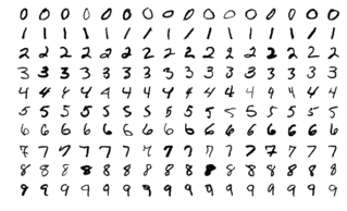
Digit Classification Exercise using Deep Learning
In this exercise, we will train our own deep learning model to solve the widely known task of digit classification. In order to do so, the trained model has to match the input and output specifications described in this documentation. The input model must be provided in ONNX format, which we will talk about in the following sections.
Instructions
- Clone the Robotics Academy repository on your local machine and checkout
noeticbranch:git clone https://github.com/JdeRobot/RoboticsAcademy cd RoboticsAcademy && git checkout noetic - Build noetic docker image. It is necessary to map the port where the camera is located to the docker container.
cd scripts docker build -f Dockerfile-noetic -t image-name . - Run docker container. It is necessary to map the port where the camera is located
- For Ubuntu: the port to map will be in /dev/videoX, you should check the number where your camera is connected.
docker run --rm -it -p 7164:7164 -p 2303:2303 -p 1905:1905 -p 8765:8765 -p 6080:6080 -p 1108:1108 --device /dev/video0:/dev/video0 jderobot/robotics-academy - For MacOs and Windows: A number of configurations must be made in order to map the ports. You can visit this documentation for it.
- For Ubuntu: the port to map will be in /dev/videoX, you should check the number where your camera is connected.
-
On the local machine navigate to 127.0.0.1:7164/ in the browser and choose the desired exercise.
-
Wait for the Connect button to turn green and display “Connected”. Click on the “Launch” button and wait for some time until an alert appears with the message
Connection Establishedand button displays “Ready”. - The exercise can be used after the alert.
Exercise Instructions
- The uploaded model should adhere to the following input/output specifications, please keep that in mind while building your model.
- The model must accept as input grayscale images with size 28x28 pixels. Input shape:
[batch_size, num_channels, height, width] = [1, 1, 28, 28] - The output must be size 10 array with the probabilities for each class. Output shape:
[batch_size, num_classes] = [1, 10]
- The model must accept as input grayscale images with size 28x28 pixels. Input shape:
- The user can train their model in any framework of their choice and export it to the ONNX format [1]. Refer to this article to know more about how to export your model. For instance, if you are working with PyTorch [2]:
import torch
model = ...
dummy_input = torch.randn(1, 1, 28, 28)
torch.onnx.export(
model, dummy_input, "mnist_cnn.onnx", verbose=True, export_params=True, input_names=['input'], output_names=['output']
)
Using the Interface
-
Browse Button: The browse button is used to browse and upload the trained deep learning model from the local machine.
-
Control Buttons: The control buttons enable the control of the interface. Play button sends the code written by User to the Image. Stop button stops the code that is currently running on the Image. Save button saves the code on the local machine. Load button loads the code from the local machine. Reset button resets the simulation (primarily, the image of the camera).
-
Brain and GUI Frequency: This input shows the running frequency of the iterative part of the code (under the
while True:). A smaller value implies the code runs less number of times. A higher value implies the code runs a large number of times. The numerator is the one set as the Measured Frequency who is the one measured by the computer (a frequency of execution the computer is able to maintain despite the commanded one) and the input (denominator) is the Target Frequency which is the desired frequency by the student. The student should adjust the Target Frequency according to the Measured Frequency. -
RTF (Real Time Factor): The RTF defines how much real time passes with each step of simulation time. A RTF of 1 implies that simulation time is passing at the same speed as real time. The lower the value the slower the simulation will run, which will vary depending on the computer.
-
Pseudo Console: This shows error messages and other logs about the exercise.
Theory
Digit classification is a classic toy example for validating machine and deep learning models. More specifically, the MNIST database of handwritten digits [3] is one of the most popular benchmarks in the literature and is widely used in tutorials as a starting point for machine learning practitioners. For solving this exercise, it is highly recommended training your model using this database.

Image classification can be achieved using classic machine learning algorithms like SVMs or Decision Trees [4]. However, these algorithms cannot compete in performance with Convolutional Neural Networks (CNNs). CNNs are a particular class of deep neural network which takes advantage of the spatial relationship between variables that are close to each other, allowing for translation invariance. In that way, they are specially suitable for processing grid-like data, such as pixels in an image or time-steps in an audio signal. CNNs are formed by subsequent convolutional layers, each of them composed of convolutional filters. The number of layers and filters has a great impact on the performance on the model, and the optimal configuration depends mostly on the particular task and the available computational resources. Other basic building blocks in CNNs are fully connected layers, activation functions and regularization strategies, such as dropout or pooling. If you are not familiarized with these concepts, here is a nice article to warm up.

For solving the particular task of digit classification, we don’t need complex architectures. Here is an example of how you can build a CNN and train a model using MNIST database with Pytorch: Basic MNIST Example. If you want to further improve the accuracy of your model, try increasing the number of layers and play around with different regularization strategies, such as data augmentation [5].
Contributors
- Contributors: David Pascual, Shashwat Dalakoti
- Maintained by David Pascual