Visual Follow Line
Goal
The goal of this exercise is to perform a PID reactive control capable of following the line painted on the racing circuit.
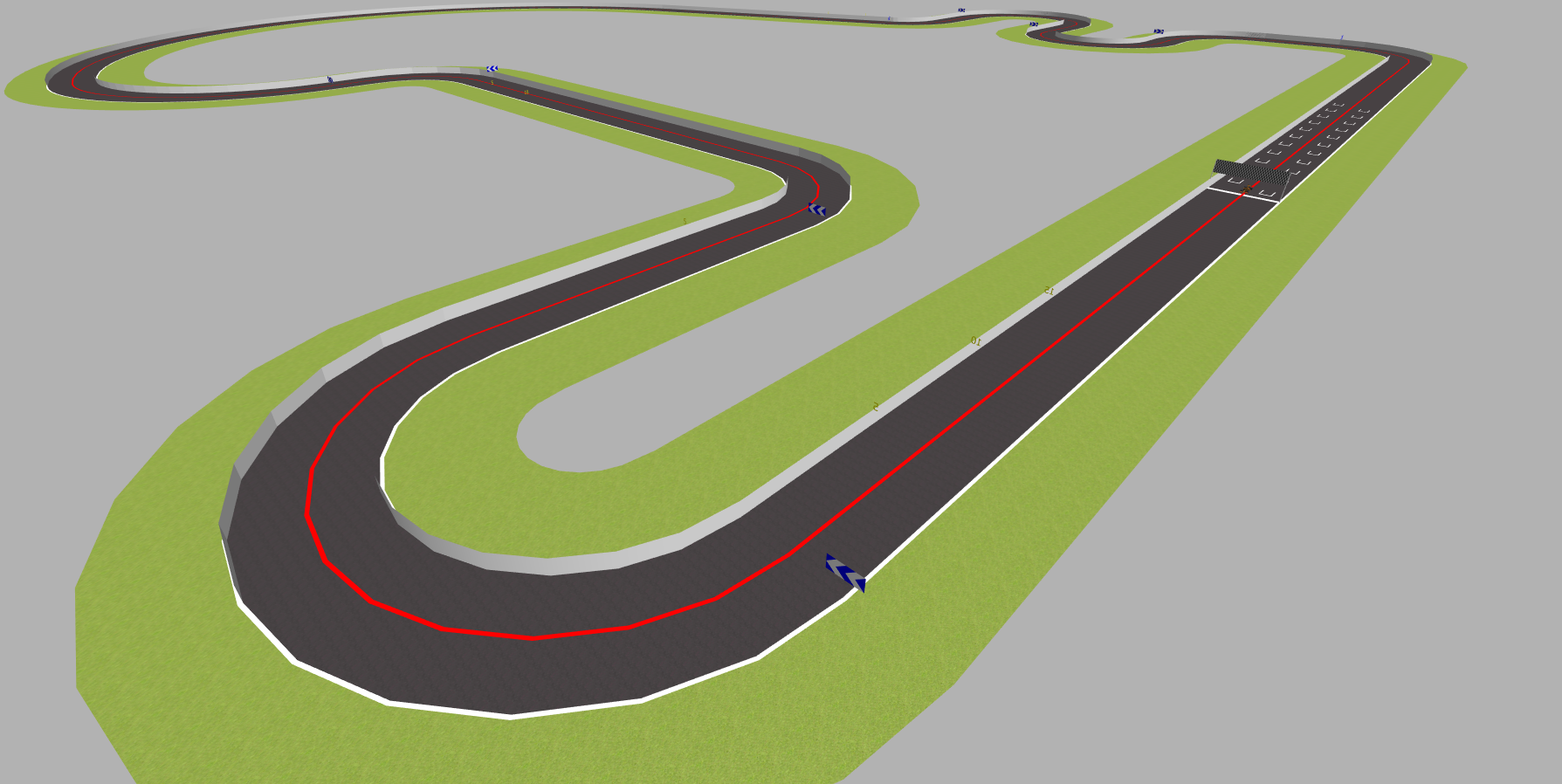
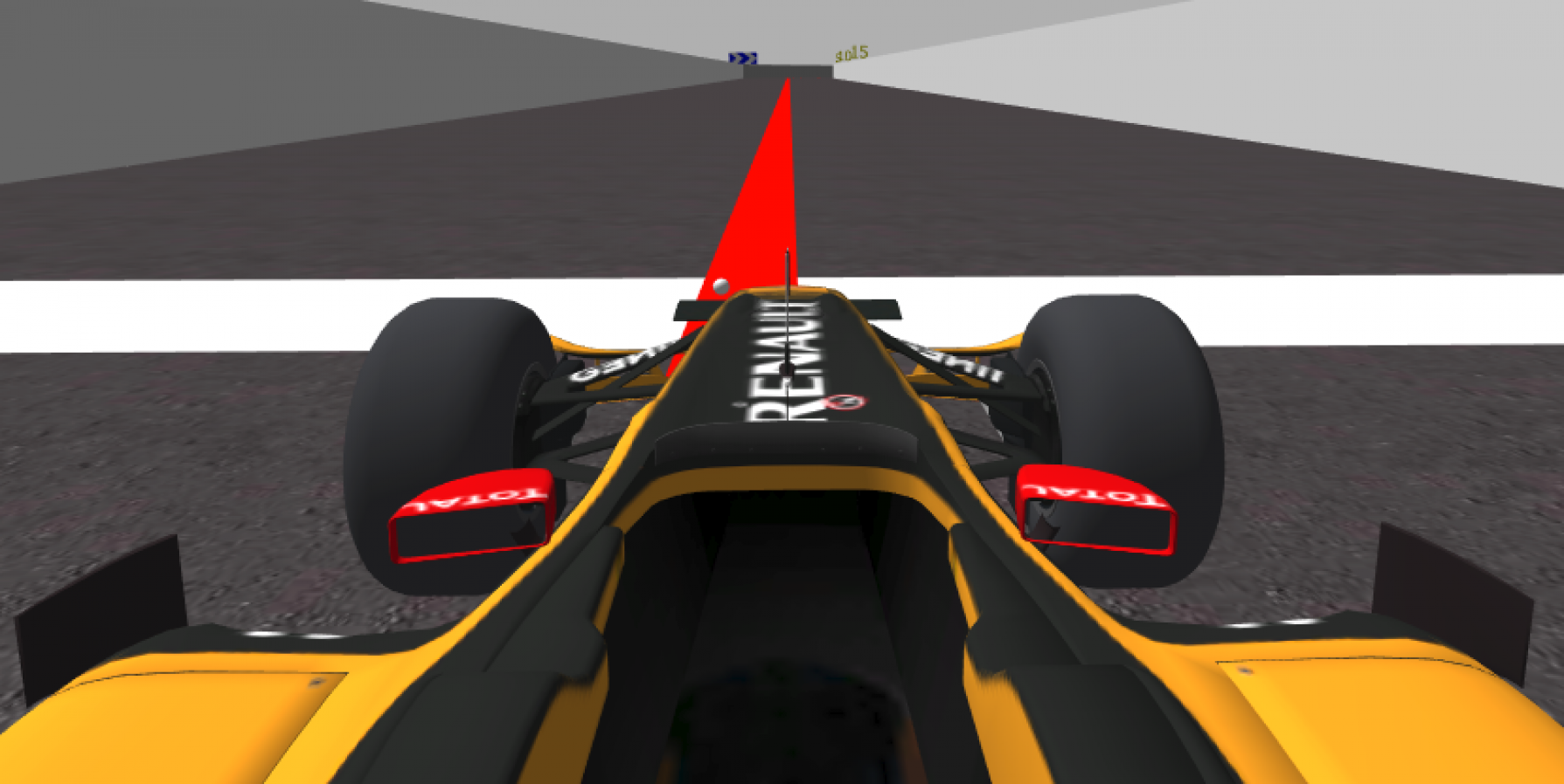
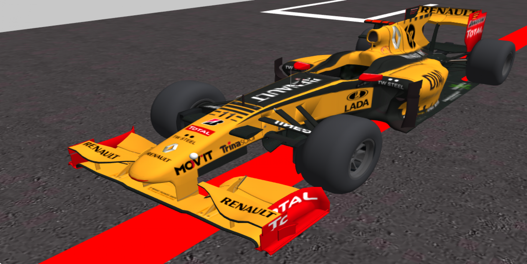
The students will program a Formula1 car in a race circuit to follow the red line in the middle of the road.
Instructions
This is the preferred way for running the exercise.
Installing and Launching
-
Download Docker. Windows users should choose WSL 2 backend Docker installation if possible, as it has better performance than Hyper-V.
-
Pull the current distribution of Robotics Academy Docker Image:
docker pull jderobot/robotics-academy:latest
-
In order to obtain optimal performance, Docker should be using multiple CPU cores. In case of Docker for Mac or Docker for Windows, the VM should be assigned a greater number of cores.
-
It is recommended to use the latest image. However, older distributions of RADI (Robotics-Academy Docker Image) can be found here.
How to perform the exercises?
-
Start a new docker container of the image and keep it running in the background:
docker run --rm -it -p 7164:7164 -p 2303:2303 -p 1905:1905 -p 8765:8765 -p 6080:6080 -p 1108:1108 -p 7163:7163 jderobot/robotics-academy -
On the local machine navigate to 127.0.0.1:7164/ in the browser and choose the desired exercise.
-
Wait for the Connect button to turn green and display “Connected”. Click on the “Launch” button and wait for some time until an alert appears with the message
Connection Establishedand button displays “Ready”. -
The exercise can be used after the alert.
Enable GPU Acceleration
- Follow the advanced launching instructions from here.
Where to insert the code?
In the launched webpage, type your code in the text editor,
from GUI import GUI
from HAL import HAL
# Enter sequential code!


while True:
    # Enter iterative code!
Using the Interface
-
Control Buttons: The control buttons enable the control of the interface. Play button sends the code written by User to the Robot. Stop button stops the code that is currently running on the Robot. Save button saves the code on the local machine. Load button loads the code from the local machine. Reset button resets the simulation(primarily, the position of the robot).
-
Brain and GUI Frequency: This input shows the running frequency of the iterative part of the code (under the
while True:). A smaller value implies the code runs less number of times. A higher value implies the code runs a large number of times. The numerator is the one set as the Measured Frequency who is the one measured by the computer (a frequency of execution the computer is able to maintain despite the commanded one) and the input (denominator) is the Target Frequency which is the desired frequency by the student. The student should adjust the Target Frequency according to the Measured Frequency. -
RTF (Real Time Factor): The RTF defines how much real time passes with each step of simulation time. A RTF of 1 implies that simulation time is passing at the same speed as real time. The lower the value the slower the simulation will run, which will vary depending on the computer.
-
Lap Time: The lap timer starts once the Robot car, moves beyond some point on the race track.
-
Pseudo Console: This shows the error messages related to the student’s code that is sent. In order to print certain debugging information on this console. The student can use the
print()command in the Editor.
Robot API
from HAL import HAL- to import the HAL(Hardware Abstraction Layer) library class. This class contains the functions that sends and receives information to and from the Hardware(Gazebo).from GUI import GUI- to import the GUI(Graphical User Interface) library class. This class contains the functions used to view the debugging information, like image widgets.HAL.getImage()- to get the imageHAL.setV()- to set the linear speedHAL.setW()- to set the angular velocityGUI.showImage()- allows you to view a debug image or with relevant information
Theory
PID Control is the main fundamental behind this exercise. To understand PID Control, let us first understand what is Control in general.
Control System
A system of devices or set of devices, that manages, commands, directs or regulates the behavior of other devices or systems to achieve the desired results. Simply speaking, a system which controls other systems. Control Systems help a robot to execute a set of commands precisely, in the presence of unforeseen errors.
Types of Control System
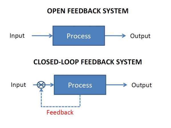
Open Loop Control System
A control system in which the control action is completely independent of the output of the system. A manual control system is on Open Loop System.
Closed Loop Control System
A control system in which the output has an effect on the input quantity in such a manner that the input will adjust itself based on the output generated. An open loop system can be converted to a closed one by providing feedback.
PID Control
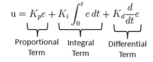
A control loop mechanism employing feedback. A PID Controller continuously calculates an error value as the difference between desired output and the current output and applies a correction based on proportional, integral and derivative terms(denoted by P, I, D respectively).
- Proportional
Proportional Controller gives an output which is proportional to the current error. The error is multiplied with a proportionality constant to get the output. And hence, is 0 if the error is 0.
- Integral
Integral Controller provides a necessary action to eliminate the offset error which is accumulated by the P Controller.It integrates the error over a period of time until the error value reaches to zero.
- Derivative
Derivative Controller gives an output depending upon the rate of change or error with respect to time. It gives the kick start for the output thereby increasing system response.

Tuning Methods
In order for the PID equation to work, we need to determine the constants of the equation. There are 3 constants called the gains of the equation. We have 2 main tuning methods for this.
- Trial and Error
It is a simple method of PID controller tuning. While system or controller is working, we can tune the controller. In this method, first we have to set Ki and Kd values to zero and increase proportional term (Kp) until system reaches to oscillating behavior. Once it is oscillating, adjust Ki (Integral term) so that oscillations stops and finally adjust D to get fast response.
- Zeigler Nichols method
Zeigler-Nichols proposed closed loop methods for tuning the PID controller. Those are continuous cycling method and damped oscillation method. Procedures for both methods are same but oscillation behavior is different. In this, first we have to set the p-controller constant, Kp to a particular value while Ki and Kd values are zero. Proportional gain is increased till system oscillates at constant amplitude.
Real Life Example
Hints
Simple hints provided to help you solve the follow_line exercise.
Detecting the Line to Follow
The first task of the assignment is to detect the line to be followed. This can be achieved easily by filtering the color of the line from the image and applying basic image processing to find the point or line to follow, or in Control terms our Set Point. Refer to these links for more information:
- https://www.pyimagesearch.com/2014/08/04/opencv-python-color-detection/
- https://stackoverflow.com/questions/10469235/opencv-apply-mask-to-a-color-image
- https://stackoverflow.com/questions/22470902/understanding-moments-function-in-opencv
Coding the Controller
The Controller can be designed in various configurations. 3 configurations have been described in detail below:
-
P Controller The simplest way to do the assignment is using the P Controller. Just find the error which is the difference between our Set Point (The point where our car should be heading) and the Current Output (Where the car is actually heading). Keep adjusting the value of the constant, till we get a value where there occurs no unstable oscillations and no slow response.
-
PD Controller This is an interesting way to see the effect of Derivative on the Control. For this, we need to calculate the derivative of the output we are receiving. Since, we are dealing with discrete outputs in our case, we simply calculate the difference between our previous error and the present error, then adjust the proportional constant. Adjust this value along with the P gain to get a good result.
-
PID Controller This is the complete implemented controller. Now, to add the I Controller we need to integrate the output from the point where error was zero, to the present output. While dealing with discrete outputs, we can achieve this using accumulated error. Then, comes the task of adjustment of gain constants till we get our desired result.
Illustrations
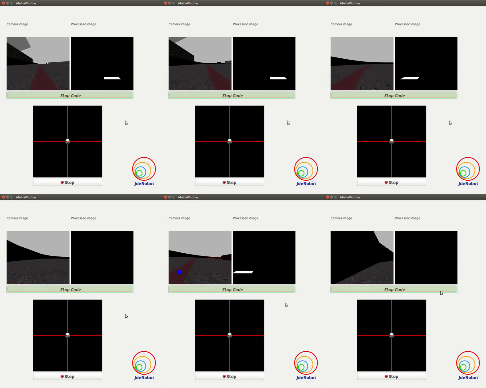
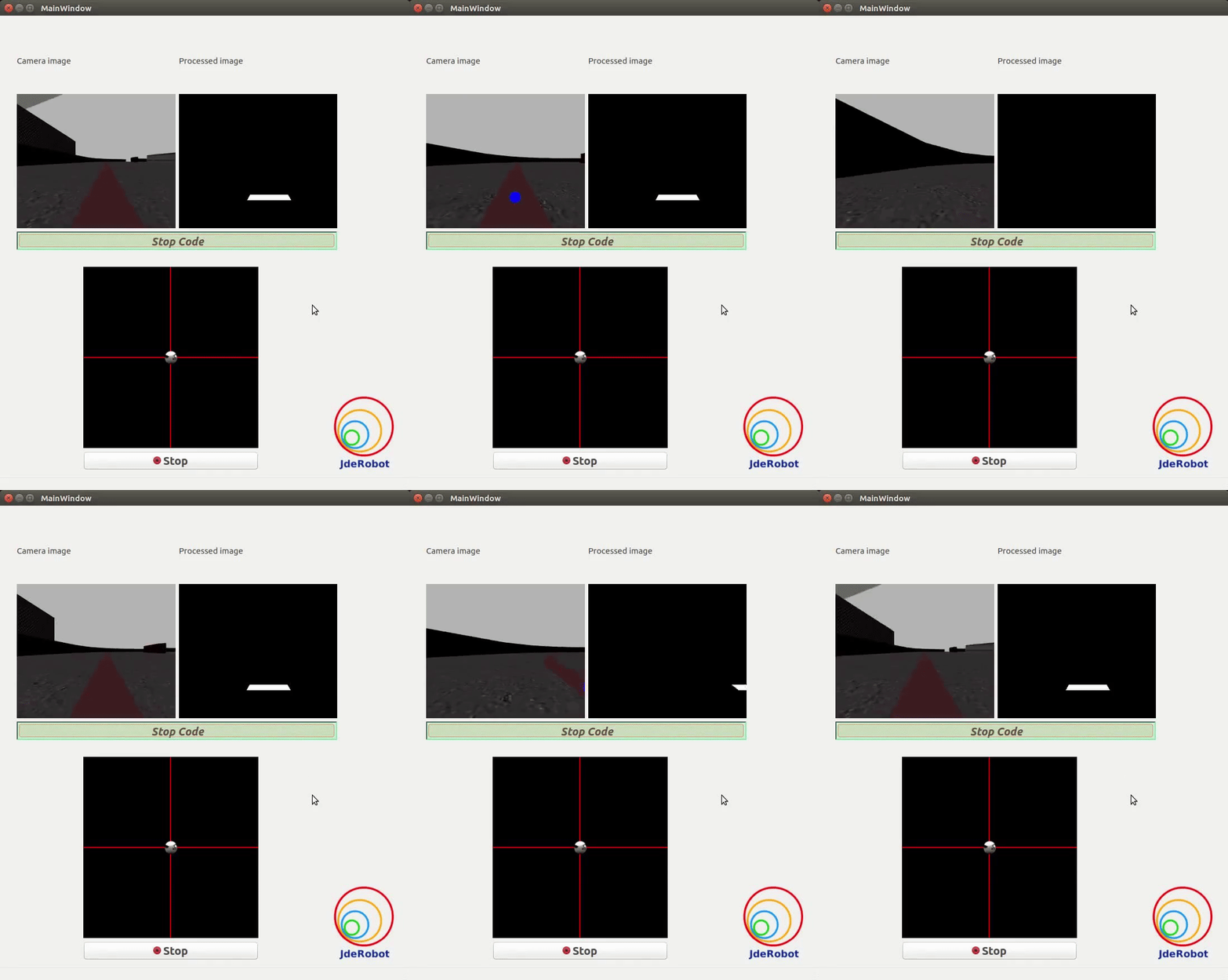
Videos
This solution is an illustration for the Web Templates
Contributors
- Contributors: Alberto Martín, Francisco Rivas, Francisco Pérez, Jose María Cañas, Nacho Arranz.
- Maintained by Pankhuri Vanjani and Sakshay Mahna.
References
- https://www.electrical4u.com/control-system-closed-loop-open-loop-control-system/
- https://en.wikipedia.org/wiki/PID_controller
- https://www.elprocus.com/the-working-of-a-pid-controller/
- https://www.tutorialspoint.com/control_systems/control_systems_introduction.htm
- https://instrumentationtools.com/open-loop-and-closed-animation-loop/
- https://trinirobotics.com/2019/03/26/arduino-uno-robotics-part-2-pid-control/
- http://homepages.math.uic.edu/~kauffman/DCalc.pdf